Revolutionizing earth observation with geospatial foundation models on AWS | Amazon Web Services

Emerging transformer-based vision models for geospatial data—also called geospatial foundation models (GeoFMs)—offer a new and powerful technology for mapping the earth’s surface at a continental scale, providing stakeholders with the tooling to detect and monitor surface-level ecosystem conditions such as forest degradation, natural disaster impact, crop yield, and many others.

GeoFMs represent an emerging research field and are a type of pre-trained vision transformer (ViT) specifically adapted to geospatial data sources. GeoFMs offer immediate value without training. The models excel as embedding models for geospatial similarity search and ecosystem change detection. With minimal labeled data, GeoFMs can be fine-tuned for custom tasks such as land surface classification, semantic segmentation, or pixel-level regression. Many leading models are available under very permissive licenses making them accessible for a wide audience. Examples include SatVision-Base, Prithvi-100M, SatMAE, and Clay (used in this solution).

In this post, we explore how Clay Foundation’s Clay foundation model, available on Hugging Face, can be deployed for large-scale inference and fine-tuning on Amazon SageMaker. For illustrative purposes, we focus on a deforestation use case from the Amazon rainforest, one of the most biodiverse ecosystems in the world. Given the strong evidence that the Amazon forest system could soon be reaching a tipping point, it presents an important domain of study and a high-impact application area for GeoFMs, for example, through early detection of forest degradation. However, the solution presented here generalizes to a wide range of geospatial use cases. It also comes with ready-to-deploy code samples to help you get started quickly with deploying GeoFMs in your own applications on AWS.

Let’s dive in!

Solution overview

At the core of our solution is a GeoFM. Architecturally, GeoFMs build on the ViT architecture first introduced in the seminal 2022 research paper An Image is Worth 16×16 Words: Transformers for Image Recognition at Scale. To account for the specific properties of geospatial data (multiple channels ranging from ultraviolet to infrared, varying electromagnetic spectrum coverage, and spatio-temporal nature of data), GeoFMs incorporate several architectural innovations such as variable input size (to capture multiple channels) or the addition of positional embeddings that capture spatio-temporal aspects such as seasonality and location on earth. The pre-training of these models is conducted on unlabeled geospatial data sampled from across the globe using masked autoencoders (MAE) as self-supervised learners. Sampling from global-scale data helps ensure that diverse ecosystems and surface types are represented appropriately in the training set. What results are general purpose models that can be used for three core use cases:

• Geospatial similarity search: Quickly map diverse surface types with semantic geospatial search using the embeddings to find similar items (such as deforested areas).
• Embedding-based change detection: Analyze a time series of geospatial embeddings to identify surface disruptions over time for a specific region.
• Custom geospatial machine learning: Fine-tune a specialized regression, classification, or segmentation model for geospatial machine learning (ML) tasks. While this requires a certain amount of labeled data, overall data requirements are typically much lower compared to training a dedicated model from the ground up.

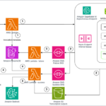
The general solution flow is shown in the following diagram. Note that this flow diagram is highly abstracted and omits certain architectural details for reasons of clarity. For a full architecture diagram demonstrating how the flow can be implemented on AWS, see the accompanying GitHub repository. This repository also contains detailed deployment instructions to get you started quickly with applying GeoFMs to your own use cases.

1. Retrieve and process satellite imagery for GeoFM inference or training: The first step is to get the raw geospatial data into a format that’s consumable by the GeoFM. This entails breaking down the large raw satellite imagery into equally-sized 256×256 pixel chips (the size that the mode expects) and normalizing pixel values, among other data preparation steps required by the GeoFM that you choose. This routine can be conducted at scale using an Amazon SageMaker AI processing job.
2. Retrieve model weights and deploy the GeoFM: Next, retrieve the open weights of the GeoFM from a model registry of your choice (HuggingFace in this example) and deploy the model for inference. The best deployment option ultimately depends on how the model is consumed. If you need to generate embedding asynchronously, use a SageMaker AI processing or transform step. For real-time inference, consider deploying to a SageMaker AI real-time endpoint, which can be configured to auto-scale with demand, allowing for large-scale inference. In this example, we use a SageMaker AI processing job with a custom Docker image for generating embeddings in batch.
3. Generate geospatial embeddings: The GeoFM is an encoder-only model, meaning that it outputs an embedding vector. During inference, you perform a forward pass of the pre-processed satellite image chip through the GeoFM. This produces the corresponding embedding vector, which can be thought of as a compressed representation of the information contained in the image. This process is equivalent to using text embedding models for RAG use cases or similar.

The generated geospatial embeddings can be used largely as-is for two key use cases: geospatial similarity search and ecosystem change detection.

4. Run similarity search on the embeddings to identify semantically similar images: The GeoFM embeddings reside in the same vector space. This allows us to identify similar items by identifying vectors that are very close to a given query point. A common high-performance search algorithm for this is approximate nearest neighbor (ANN). For scalability and search performance, we index the embedding vectors in a vector database.
5. Analyze time-series of embeddings for break points that indicate change: Instead of looking for similarity between embedding vectors, you can also look for distance. Doing this for a specific region and across time lets you pinpoint specific times where change occurs. This allows you to use embeddings for surface change detection over time, a very common use case in geospatial analytics.

Optionally, you can also fine-tune a model on top of the GeoFM.

6. Train a custom head and run inference: To fine-tune a model you add a custom (and typically lightweight) head on top of the GeoFM and fine-tune it on a (often small) labeled dataset. The GeoFM weights remain frozen and are not retrained. The custom head takes the GeoFM-generated embedding vectors as input and produces classification masks, pixel-level recessions results, or simply a class per image, depending on the use case.

We explore the key steps of this workflow in the next sections. For additional details on the implementation—including. how to build a high-quality user interface with Solara—see the accompanying GitHub repository.

Geospatial data processing and embedding generation

Our comprehensive, four-stage data processing pipeline transforms raw satellite imagery into analysis-ready vector embeddings that power advanced geospatial analytics. This orchestrated workflow uses Amazon SageMaker AI Pipelines to create a robust, reproducible, and scalable processing architecture. The end-to-end solution can process Earth observation data for a selected region of interest, with built-in flexibility to adapt to different use cases. In this example, we use Sentinel-2 imagery from the Amazon Registry of Open Data for monitoring deforestation in the Brazilian rainforest. However, our pipeline architecture is designed to work seamlessly with other satellite image providers and resolutions (such as NAIP with 1m/pixel resolution, or Maxar and Planet Labs up to below 1m/pixel resolution).

Pipeline architecture overview

The SageMaker pipeline consists of four processing steps, shown in the preceding figure, each step builds on the outputs of the previous steps with intermediate results stored in Amazon Simple Storage Service (Amazon S3).

1. Pre-process satellite tiles: Divides the satellite imagery into chips. We chose a chip size of 256×256 pixels as expected by Clay v1. For Sentinel-2 images this corresponds to an area of 2.56 x 2.56 km².
2. Generate embeddings: Creates 768-dimensional vector representations for the chips using the Clay v1 model.
3. Process embeddings: Performs dimensionality reduction and computes similarity metrics (for downstream analyses).
4. Consolidate and index: Consolidates outputs and loads embeddings vectors into a Vector store.

# Pipeline definition (simplified)
pipeline = Pipeline(
    name=f"EmbeddingPipeline-{aoi_name}",
    steps=[preprocess_step, embeddings_step, postprocessing_step, consolidation_step],
    parameters=[bucket_name_param, aoi_name_param, s2_grid_id_param, 
               chip_size_param, batch_size_param, s2_bands_param],
    sagemaker_session=pipeline_session
)

Step 1: Satellite data acquisition and chipping

The pipeline starts by accessing Sentinel-2 multispectral satellite imagery through the AWS Open Data program from S3 buckets. This imagery provides 10-meter resolution across multiple spectral bands including RGB (visible light) and NIR (near-infrared), which are critical for environmental monitoring.

This step filters out chips that have excessive cloud cover and divides large satellite scenes into manageable 256×256 pixel chips, which enables efficient parallel processing and creates uniform inputs for the foundation model. This step also runs on a SageMaker AI Processing job with a custom Docker image optimized for geospatial operations.

# Chip generation – Simplified version
def generate_chips_from_xarray(ds, chip_size, aoi_name, s2_scene_id):
    """Generates image chips of specified size from xarray dataset
       using Area of Interest (AOI) name and Sentinel-2 scene id"""
    try:
        # Calculate optimal number of jobs for parallel processing
        n_jobs = min(os.cpu_count(), 16)  # Use optimal number of cores or available CPU count
        logger.info(f"Using {n_jobs} parallel jobs for chip generation")
        
        # Generate all x,y coordinates for processing
        coordinates = [(x, y) 
                    for x in range(0, ds.sizes['x'], chip_size)
                    for y in range(0, ds.sizes['y'], chip_size)]
        
        logger.info(f"Generating {len(coordinates)} chips from scene")
        
        # Process chips in parallel
        with parallel_backend('threading', n_jobs=n_jobs):
            results = Parallel(verbose=1)(
                delayed(process_single_chip)(
                    x, y, ds, chip_size, s2_scene_id
                ) for x, y in coordinates
            )
        
        # Filter out None results (e.g., chips with too many cloud pixels)
        valid_results = [r for r in results if r is not None]
        
        logger.info(f"Successfully generated {len(valid_results)} valid chips")
        
        return valid_results
    except Exception as e:
        logger.error(f"Error in chip generation for scene {s2_scene_id}: {str(e)}")
        raise

For each chip, this step generates:

• NetCDF datacubes (.netcdf) containing the full multispectral information
• RGB thumbnails (.png) for visualization
• Rich metadata (.parquet) with geolocation, timestamps, and other metadata

Step 2: Embedding generation using a Clay foundation model

The second step transforms the preprocessed image chips into vector embeddings using the Clay v1 foundation model. This is the most computationally intensive part of the pipeline, using multiple GPU instances (ml.g5.xlarge) to efficiently process the satellite imagery.

For each chip, this step:

• Accesses the NetCDF datacube from Amazon S3
• Normalizes the spectral bands according to the Clay v1 model’s input requirements
• Generates both patch-level and class token (CLS) embeddings
• Stores the embeddings as NumPy arrays (.npy) alongside the original data on S3 as intermediate store

While Clay can use all Sentinel-2 spectral bands, our implementation uses RGB and NIR as input bands to generate a 768-dimensional embedding, which provide excellent results in our examples. Customers can easily adapt the input bands based on their specific use-cases. These embeddings encapsulate high-level features such as vegetation patterns, urban structures, water bodies, and land use characteristics—without requiring explicit feature engineering.

Step 3: Embedding processing and analysis

The third step analyzes the embeddings to extract meaningful insights, particularly for time-series analysis. Running on high-memory instances, this step:

1. Performs dimensionality reduction on the embeddings using principal component analysis (PCA) and t-distributed stochastic neighbor embedding (t-SNE) (to be used later for change detection)
2. Computes cosine similarity between embeddings over time (an alternative for change detection)
3. Identifies significant changes in the embeddings that might indicate surface changes
4. Saves processed embeddings in Parquet format for efficient querying

The output includes processed embedding files that contain both the original high-dimensional vectors and their reduced representations, along with computed similarity metrics.

For change detection applications, this step establishes a baseline for each geographic location and calculates deviations from this baseline over time. These deviations, captured as vector distances, provide a powerful indicator of surface changes like deforestation, urban development, or natural disasters.

Step 4: Consolidation and vector database integration

The final pipeline step consolidates the processed embeddings into a unified dataset and loads them into vector databases optimized for similarity search. The outputs include consolidated embedding files, GeoJSON grid files for visualization, and configuration files for frontend applications.

The solution supports two vector database options:

Both options provide efficient ANN search capabilities, enabling sub-second query performance. The choice between them depends on the scale of deployment, integration requirements, and operational preferences.

With this robust data processing and embedding generation foundation in place, let’s explore the real-world applications enabled by the pipeline, beginning with geospatial similarity search.

Geospatial similarity search

Organizations working with Earth observation data have traditionally struggled with efficiently identifying specific landscape patterns across large geographic regions. Traditional Earth observation analysis requires specialized models trained on labeled datasets for each target feature. This approach forces organizations into a lengthy process of data collection, annotation, and model training before obtaining results.

In contrast, the GeoFM-powered similarity search converts satellite imagery into 768-dimensional vector embeddings that capture the semantic essence of landscape features, eliminating the need for manual feature engineering and computation of specialized indices like NDVI or NDWI.

This capability uses the Clay foundation model’s pre-training on diverse global landscapes to understand complex relationships between features without explicit programming. The result is an intuitive image-to-image search capability where users can select a reference area—such as early-stage deforestation or wildfire damage—and instantly find similar patterns across vast territories in seconds rather than weeks.

Similarity search implementation

Our implementation provides a streamlined workflow for finding similar geographic areas using the embeddings generated by the data processing pipeline. The search process involves:

1. Reference area selection: Users select a reference chip representing a search term (for example, a deforested patch, urban development, or agricultural field)
2. Search parameters: Users specify the number of results and a similarity threshold
3. Vector search execution: The system retrieves similar chips using cosine similarity between embeddings
4. Result visualization: Matching chips are highlighted on the map

Let’s dive deeper on a real-world application, taking our running example of detecting deforestation in the Mato Grosso region of the Brazilian Amazon. Traditional monitoring approaches often detect forest loss too late—after significant damage has already occurred. The Clay-powered similarity search capability offers a new approach by enabling early detection of emerging deforestation patterns before they expand into large-scale clearing operations.

Using a single reference chip showing the initial signs of forest degradation—such as selective logging, small clearings, or new access roads—analysts can instantly identify similar patterns across vast areas of the Amazon rainforest. As demonstrated in the following example images, the system effectively recognizes the subtle signatures of early-stage deforestation based on a single reference image. This capability enables environmental protection agencies and conservation organizations to deploy resources precisely, improving the anti-deforestation efforts by addressing threats to prevent major forest loss. While a single reference chip image led to good results in our examples, alternative approaches exist, such as an average vector strategy, which leverages embeddings from multiple reference images to enhance the similarity search results.

Ecosystem change detection

Unlike vector-based similarity search, change detection focuses on measuring the distance between embedding vectors over time, the core assumption being that the more distant embedding vectors are to each other, the more dissimilar the underlying satellite imagery is. If applied to a single region over time, this lets you pinpoint so called change points—periods where significant and long-lasting change in surface conditions occurred.

Our solution implements a timeline view of Sentinel-2 satellite observations from 2018 to present. Each observation point corresponds to a unique satellite image, allowing for detailed temporal analysis. While embedding vectors are highly dimensional, we use the previously computed PCA (and optionally t-SNE) to reduce dimensionality to a single dimension for visualization purposes.

Let’s review a compelling example from our analysis of deforestation in the Amazon. The following image is a timeseries plot of geospatial embeddings (first principal component) for a single 256×256 pixel chip. Cloudy images and major outliers have been removed.

Points clustered closely on the y-axis indicate similar ground conditions; sudden and persistent discontinuities in the embedding values signal significant change. Here’s what the analysis shows:

• Stable forest conditions from 2018 through 2020
• A significant discontinuity in embedding values during 2021. Closer review of the underlying satellite imagery shows clear evidence of forest clearing and conversion to agricultural fields
• Further transformation visible in 2024 imagery

Naturally, we need a way to automate the process of change detection so that it can be applied at scale. Given that we do not typically have extensive changepoint training datasets, we need an unsupervised approach that works without labeled data. The intuition behind unsupervised change detection is the following: identify what normal looks like, then highlight large enough deviations from normal and flag them as change points; after a change point has occurred, characterize the new normal and repeat the process.

The following function performs harmonic regression analysis on the embeddings timeseries data, specifically designed to model yearly seasonality patterns. The function fits a harmonic regression with a specified frequency (default 365 days for annual patterns) to the embedding data of a baseline period (the year 2018 in this example). It then generates predictions and calculates error metrics (absolute and percentage deviations). Large deviations from the normal seasonal pattern indicate change and can be automatically flagged using thresholding.

def fit_harmonic_regression(data, outliers, date_col="date", y_col="patch_emb_pca_1", 
                          baseline_start_date=datetime.datetime(2018,1,1), 
                          monitoring_start_date=datetime.datetime(2019,1,1), 
                          deg=3, reg=0.001, avg_days_yr=365):
    """
    Fits a harmonic regression model to time series data using Lasso regularization.
    
    Parameters:
    - data: DataFrame containing the time series data
    - outliers: List of dates to exclude from the fitting process
    - date_col: Name of the column containing dates (default: 'date')
    - y_col: Name of the column containing target values (default: 'patch_emb_pca_1')
    - baseline_start_date: Start date for the baseline period (default: Jan 1, 2018)
    - monitoring_start_date: Start date for the monitoring period (default: Jan 1, 2019)
    - deg: Degree of polynomial features (default: 3)
    - reg: Regularization strength for Lasso (default: 0.001)
    - avg_days_yr: Number of days in a year (default: 365)
    """

    # Convert date column to datetime format and create numerical representation
    data[date_col] = pd.to_datetime(data[date_col])
    data["date_numerical"] = data[date_col].apply(lambda x: mdates.date2num(x))
    t_full = data["date_numerical"]
    y_full = data[y_col]
    
    # Filter data for model fitting:
    # - Remove outliers
    # - Keep only data between baseline_start_date and monitoring_start_date
    t_fitting = data[
        (~data["date"].isin(outliers)) & 
        (data[date_col] >= baseline_start_date) & 
        (data[date_col] < monitoring_start_date)
    ]["date_numerical"]
    
    y_fitting = data[
        (~data["date"].isin(outliers)) & 
        (data[date_col] >= baseline_start_date) & 
        (data[date_col] < monitoring_start_date)
    ][y_col]
    
    # Create design matrix for harmonic regression
    # Convert time to angular frequency (2π/period)
    w = 2 * np.pi / avg_days_yr
    
    # Generate polynomial features from sine and cosine transformations
    poly = PolynomialFeatures(deg)
    # Create feature matrix for fitting period
    X_fitting = poly.fit_transform(np.column_stack((
        np.sin(w*t_fitting), 
        np.cos(w*t_fitting)
    )))
    # Create feature matrix for all data points
    X_full = poly.fit_transform(np.column_stack((
        np.sin(w*t_full), 
        np.cos(w*t_full)
    )))

    # Initialize and fit Lasso regression model
    lasso_model = Lasso(alpha=reg)
    lasso_model.fit(X_fitting, y_fitting)
    
    # Generate predictions for all time points
    y_fit = lasso_model.predict(X_full)
    
    # Calculate error metrics
    absolute_deviation = np.abs(y_full - y_fit)
    percentage_deviation = (absolute_deviation / np.abs(y_fit)) * 100
    
    # Compile results into a DataFrame
    df = pd.DataFrame()
    df["date"] = data[date_col]
    df["date_numerical"] = data["date_numerical"] 
    df[f"{y_col}_true"] = data[y_col]          # Original values
    df[f"{y_col}_pred"] = y_fit                # Predicted values
    df[f"{y_col}_abs_error"] = absolute_deviation    # Absolute error
    df[f"{y_col}_perc_error"] = percentage_deviation # Percentage error
    # Add time-based features
    df["year"] = df["date"].apply(lambda x: x.year)
    df["month"] = df["date"].apply(lambda x: x.month)
    df["year_month"] = df.apply(
        lambda x: "{}_{}".format(str(x.year), str(x.month)), 
        axis=1
    )
    # Return the fitted model, polynomial transformer, and results DataFrame
    return lasso_model, poly, df

When applied to the chips across an area of observation and defining a threshold on the maximum deviation from the fitted harmonic regression, we can automatically map change intensity allowing analysts to quickly zoom in on problematic areas.

While this method performs well in our analyses, it is also quite rigid in that it requires a careful tuning of error thresholds and the definition of a baseline period. There are more sophisticated approaches available ranging from general-purpose time-series analyses that automate the baseline definition and change point detection using recursive methods (for example, Gaussian Processes) to specialized algorithms for geospatial change detection (for example, LandTrendr, and Continuous Change Detection and Classification (CCDC)).

In sum, our approach to change detection demonstrates the power of geospatial embedding vectors in tracking environmental changes over time, providing valuable insights for land use monitoring, environmental protection, and urban planning applications.

GeoFM fine-tuning for your custom use case

Fine-tuning is a specific implementation of transfer learning, in which a pre-trained foundation model is adapted to specific tasks through targeted additional training on specialized labeled datasets. For GeoFMs, these specific tasks can target agriculture, disaster monitoring or urban analysis. The model retains its broad spatial understanding while developing expertise for particular regions, ecosystems or analytical tasks. This approach significantly reduces computational and data requirements compared to building specialized models from scratch, without sacrificing accuracy. Fine-tuning typically involves preserving the pre-trained Clay’s encoder—which has already learned rich representations of spectral patterns, spatial relationships, and temporal dynamics from massive satellite imagery, while attaching and training a specialized task-specific head.

For pixel-wise prediction tasks—such as land use segmentation—the specialized head is typically a decoder architecture, whereas for class-level outputs (classification tasks) the head can be as basic as a multilayer perceptron network. Training focuses exclusively on the new decoder that captures the feature representations from model’s frozen encoder and gradually transforms them back to full-resolution images where each pixel is classified according to its land use type.

The segmentation framework combines the powerful pre-trained Clay encoder with an efficient convolutional decoder, taking Clay’s rich understanding of satellite imagery and converting it into detailed land use maps. The lightweight decoder features convolutional layers and pixel shuffle upsampling techniques that capture the feature representations from Clay’s frozen encoder and gradually transforms them back to full-resolution images where each pixel is classified according to its land use type. By freezing the encoder (which contains 24 transformer heads and 16 attention heads) and only training the compact decoder, the model achieves a good balance between computational efficiency and segmentation accuracy.

We applied this segmentation architecture on a labeled land use land cover (LULC) dataset from Impact Observatory and hosted on the Amazon Registry of Open Data. For illustrative purposes, we again focused on our running example from Brazil’s Mato Grosso region. We trained the decoder head for 10 epochs which took 17 minutes total and tracked intersection over union (IOU) and F1 score as segmentation accuracy metrics. After just one training epoch, the model already achieved 85.7% validation IOU. With the full 10 epochs completed, performance increased to an impressive 92.4% IOU and 95.6% F1 score. In the following image, we show ground truth satellite imagery (upper) and the model’s predictions (lower). The visual comparison highlights how accurately this approach can classify different land use categories.

Conclusion

Novel GeoFMs provide an encouraging new approach to geospatial analytics. Through their extensive pre-training, these models have incorporated a deep implicit understanding of geospatial data and can be used out-of-the-box for high-impact use cases such as similarity search or change detection. They can also serve as the basis for specialized models using a fine-tuning process that is significantly less data-hungry (fewer labeled data needed) and has lower compute requirements.

In this post, we have shown how you can deploy a state-of-the-art GeoFM (Clay) on AWS and have explored one specific use case – monitoring deforestation in the Amazon rainforest – in greater detail. The same approach is applicable to a large variety of industry use case. For example, insurance companies can use a similar approach to ours to assess damage after natural disasters including hurricanes, floods or fires and keep track of their insured assets. Agricultural organizations can use GeoFMs for crop type identification, crop yield predictions, or other use cases. We also envision high-impact use cases in industries like urban planning, emergency and disaster response, supply chain and global trade, sustainability and environmental modeling, and many others. To get started applying GeoFMs to your own earth observation use case, check out the accompanying GitHub repository, which has the prerequisites and a step-by-step walkthrough to run it on your own area of interest.

About the Authors

Dr. Karsten Schroer is a Senior Machine Learning (ML) Prototyping Architect at AWS, focused on helping customers leverage artificial intelligence (AI), ML, and generative AI technologies. With deep ML expertise, he collaborates with companies across industries to design and implement data- and AI-driven solutions that generate business value. Karsten holds a PhD in applied ML.

Bishesh Adhikari is a Senior ML Prototyping Architect at AWS with over a decade of experience in software engineering and AI/ML. Specializing in GenAI, LLMs, NLP, CV, and GeoSpatial ML, he collaborates with AWS customers to build solutions for challenging problems through co-development. His expertise accelerates customers’ journey from concept to production, tackling complex use cases across various industries. In his free time, he enjoys hiking, traveling, and spending time with family and friends.

Dr. Iza Moise is a Senior Machine Learning (ML) Prototyping Architect at AWS, with expertise in both traditional ML and advanced techniques like foundation models and vision transformers. She focuses on applied ML across diverse scientific fields, publishing and reviewing at Amazon’s internal ML conferences. Her strength lies in translating theoretical advances into practical solutions that deliver measurable impact through thoughtful implementation.